Alumni Contributions
Data Mining and Business Analytics with R
This is a summary of example 2 in Chapter 2 of the book “Data Mining and Business Analytics with R”. The post keeps the original code with some polishing syntax for better plotting, particularly using ggplot2 package and gridExtra.
Code and Data are saved in Github link
library(lattice)
library(ggplot2)
#Using multiple plot function when using with ggplot
#source("https://raw.githubusercontent.com/namkyodai/BusinessAnalytics/master/genericfunctions/multiplot.R")
#----1. Data
don <- read.csv("contribution.csv")
#or read directly from the web
#don <- read.csv("https://www.biz.uiowa.edu/faculty/jledolter/DataMining/contribution.csv")
#or
don[1:5,] #display the first 5 data rows
table(don$Class.Year) #display total numbers of data points for each batch of year
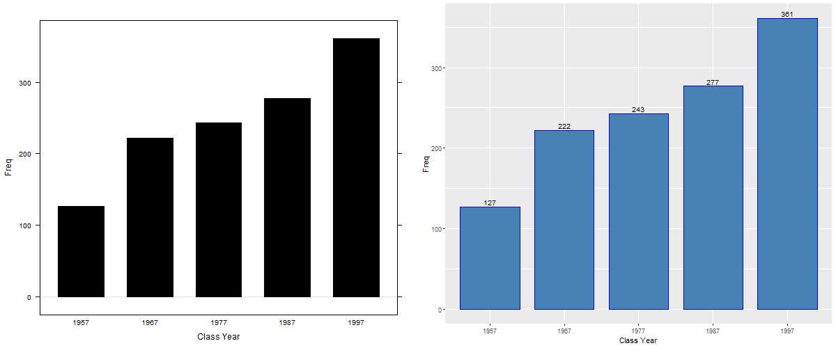
a=barchart(table(don$Class.Year),horizontal=FALSE,xlab="Class Year",col="black")
p=ggplot(data.frame(table(don$Class.Year)), aes(x=Var1, y=Freq))+labs(y="Freq", x="Class Year") + geom_bar(stat="identity",width=0.8,color="blue",fill="steelblue")+geom_text(aes(label=Freq), vjust=-0.3, size=3.5)
plot.new()
par(mar=c(4.5,4.3,1,1)+0.1,mfrow=c(1,2),bg="white")
library(gridExtra) #this package allows to plot multiple graphs in the same plot despite the difference in plotting engines (e.g. ggplot or barchart)
grid.arrange(a, p, ncol = 2) #display the two plot a and p
dev.copy(png,'alumni_classyear_bar.png',width = 1200, height = 500)
dev.off()
> don[1:5,]
  Gender Class.Year Marital.Status   Major Next.Degree FY04Giving FY03Giving FY02Giving
1      M       1957              M History         LLB       2500       2500       1400
2      M       1957              M Physics          MS       5000       5000       5000
3      F       1957              M   Music        NONE       5000       5000       5000
4      M       1957              M History        NONE          0       5100        200
5      M       1957              M Biology          MD       1000       1000       1000
  FY01Giving FY00Giving AttendenceEvent
1      12060      12000               1
2       5000      10000               1
3       5000      10000               1
4        200          0               1
5       1005       1000               1
> table(don$Class.Year)

1957 1967 1977 1987 1997
 127  222  243  277  361
Barchart from Lattice package
don$TGiving=don$FY00Giving+don$FY01Giving+don$FY02Giving+don$FY03Giving+don$FY04Giving
mean(don$TGiving)
sd(don$TGiving)
quantile(don$TGiving,probs=seq(0,1,0.05))
quantile(don$TGiving,probs=seq(0.95,1,0.01))
mean(don$TGiving)
[1] 980.0436
> sd(don$TGiving)
[1] 6670.773
> quantile(don$TGiving,probs=seq(0,1,0.05))
      0%       5%      10%      15%      20%      25%      30%      35%      40%      45%
     0.0      0.0      0.0      0.0      0.0      0.0      0.0     10.0     25.0     50.0
     50%      55%      60%      65%      70%      75%      80%      85%      90%      95%
    75.0    100.0    150.8    200.0    275.0    400.0    554.2    781.0   1050.0   2277.5
    100%
171870.1
> quantile(don$TGiving,probs=seq(0.95,1,0.01))
      95%       96%       97%       98%       99%      100%
  2277.50   3133.56   5000.00   7000.00  16442.14 171870.06
#---------------------
plot.new()
par(mar=c(4.5,4.3,1,1)+0.1,mfrow=c(2,2))
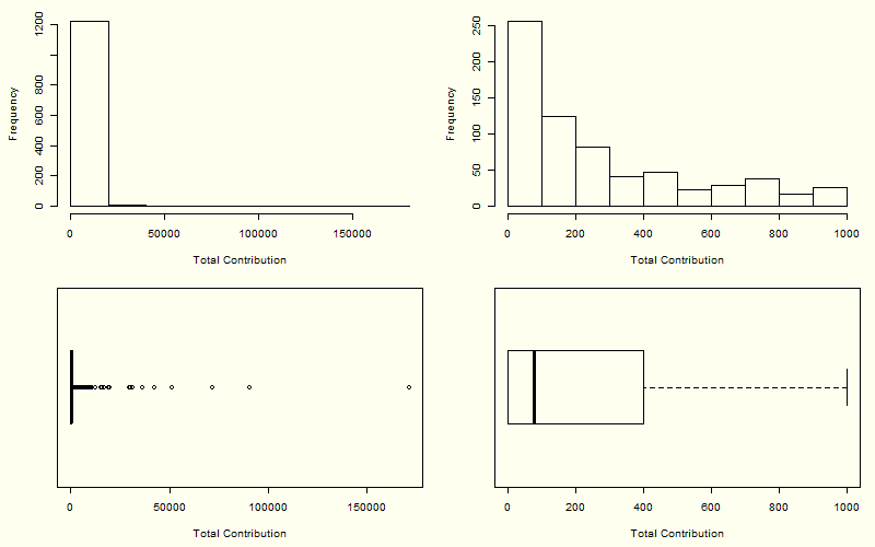
hist(don$TGiving,main=NULL,xlab="Total Contribution") #histograph with outliners
hist(don$TGiving[don$TGiving!=0][don$TGiving[don$TGiving!=0]<=1000],main=NULL,xlab="Total Contribution") #histograph after delete outliners
boxplot(don$TGiving,horizontal=TRUE,xlab="Total Contribution") #boxplot with outliners
boxplot(don$TGiving,outline=FALSE,horizontal=TRUE,xlab="Total Contribution") #boxplot without outliners
dev.copy(png,'alumni_contributionplot.png',width = 800, height = 500)
dev.off()
ddd=don[don$TGiving>=30000,] #seeing only total giving greater than 30K
ddd
ddd1=ddd[,c(1:5,12)] #display colum from 1 to 5 and column 12
ddd1
ddd1[order(ddd1$TGiving,decreasing=TRUE),] #display with decreasing
#-----------------
plot.new()
par(mar=c(4.5,4.3,1,1)+0.1,mfrow=c(2,2))
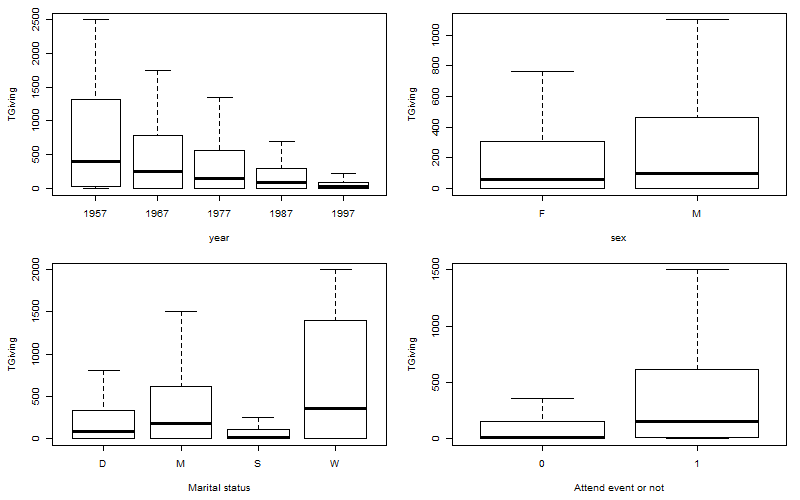
boxplot(TGiving~Class.Year,data=don,outline=FALSE, xlab="year")
boxplot(TGiving~Gender,data=don,outline=FALSE, xlab="sex")
boxplot(TGiving~Marital.Status,data=don,outline=FALSE,xlab="Marital status")
boxplot(TGiving~AttendenceEvent,data=don,outline=FALSE,xlab="Attend event or not")
dev.copy(png,'alumni_distribution_boxplot.png',width = 800, height = 500)
dev.off()
plot.new()
#-----------------
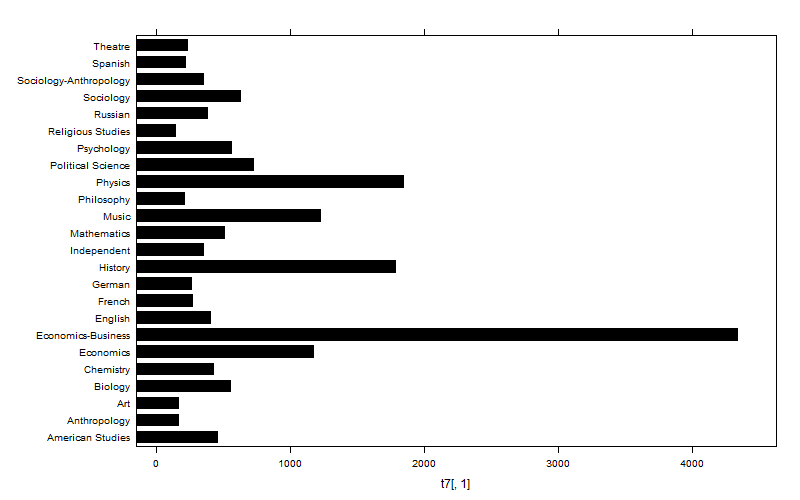
t4=tapply(don$TGiving,don$Major,mean,na.rm=TRUE)
t4
t5=table(don$Major)
t5
t6=cbind(t4,t5)
t7=t6[t6[,2]>10,]
t7[order(t7[,1],decreasing=TRUE),]
plot(barchart(t7[,1],col="black"))
dev.copy(png,'alumni_major_barplot.png',width = 800, height = 500)
dev.off()
#-----------------
plot.new()
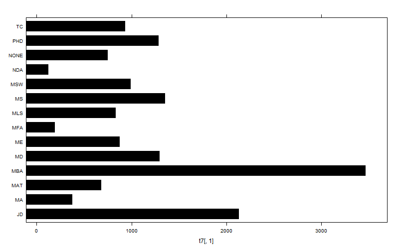
t4=tapply(don$TGiving,don$Next.Degree,mean,na.rm=TRUE)
t4
t5=table(don$Next.Degree)
t5
t6=cbind(t4,t5)
t7=t6[t6[,2]>10,]
t7[order(t7[,1],decreasing=TRUE),]
plot(barchart(t7[,1],col="black"))
dev.copy(png,'alumni_degree_barplot.png',width = 800, height = 500)
dev.off()
#-----------------
plot.new()
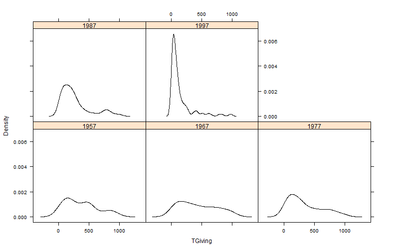
densityplot(~TGiving|factor(Class.Year),data=don[don$TGiving<=1000,][don[don$TGiving<=1000,]$TGiving>0,],plot.points=FALSE,col="black")
dev.copy(png,'alumni_year_densityplot.png',width = 800, height = 500)
dev.off()
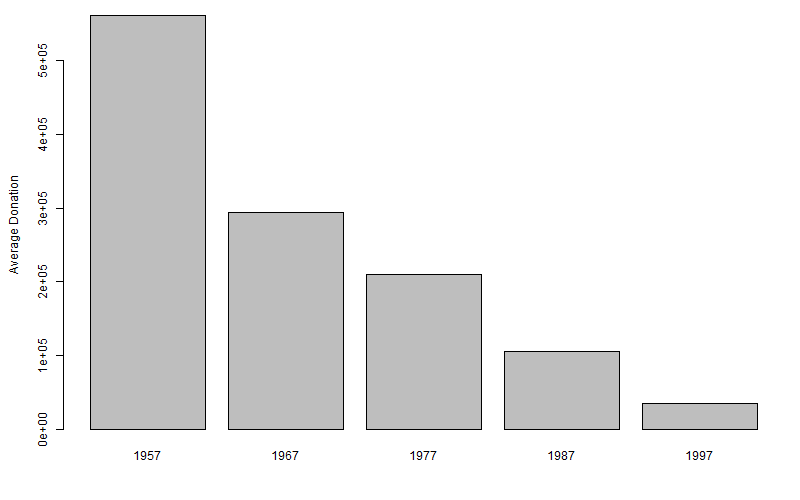
t11=tapply(don$TGiving,don$Class.Year,FUN=sum,na.rm=TRUE)
t11
#-----------------
plot.new()
par(mfrow=c(1,1))
barplot(t11,ylab="Average Donation")
dev.copy(png,'alumni_year_barplot.png',width = 800, height = 500)
dev.off()
#-----------------
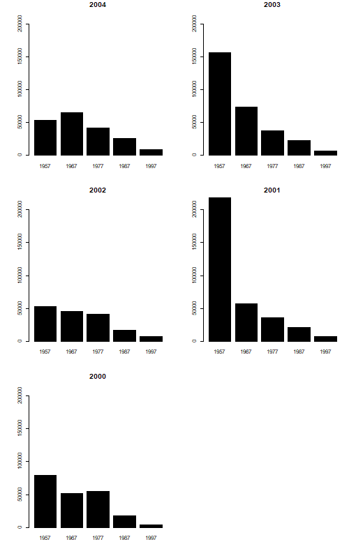
plot.new()
par(mar=c(4.5,4.3,1,1)+0.1,mfrow=c(2,2))
barchart(tapply(don$FY04Giving,don$Class.Year,FUN=sum,
na.rm=TRUE),horizontal=FALSE,ylim=c(0,225000),col="black", main="2004")
barchart(tapply(don$FY03Giving,don$Class.Year,FUN=sum,
na.rm=TRUE),horizontal=FALSE,ylim=c(0,225000),col="black", main="2003")
barchart(tapply(don$FY02Giving,don$Class.Year,FUN=sum,
na.rm=TRUE),horizontal=FALSE,ylim=c(0,225000),col="black", main="2002")
barchart(tapply(don$FY01Giving,don$Class.Year,FUN=sum,
na.rm=TRUE),horizontal=FALSE,ylim=c(0,225000),col="black", main="2001")
barchart(tapply(don$FY00Giving,don$Class.Year,FUN=sum,
na.rm=TRUE),horizontal=FALSE,ylim=c(0,225000),col="black", main="2000")
#same plot but with par
#-----------------
plot.new()
par(mar=c(4.5,4.3,1,1)+0.1,mfrow=c(3,2),bg="white")
barplot(tapply(don$FY04Giving,don$Class.Year,FUN=sum,
na.rm=TRUE),ylim=c(0,225000),col="black", main="2004")
barplot(tapply(don$FY03Giving,don$Class.Year,FUN=sum,
na.rm=TRUE),ylim=c(0,225000),col="black", main="2003")
barplot(tapply(don$FY02Giving,don$Class.Year,FUN=sum,
na.rm=TRUE),ylim=c(0,225000),col="black", main="2002")
barplot(tapply(don$FY01Giving,don$Class.Year,FUN=sum,
na.rm=TRUE),ylim=c(0,225000),col="black", main="2001")
barplot(tapply(don$FY00Giving,don$Class.Year,FUN=sum,
na.rm=TRUE),ylim=c(0,225000),col="black", main="2000")
dev.copy(png,'alumni_annual_barplot.png',width = 500, height = 800)
dev.off()
#-----------------
plot.new()
par(mfrow=c(1,1))
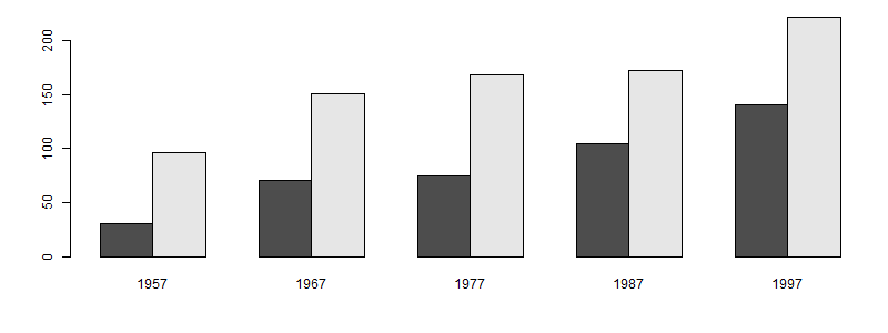
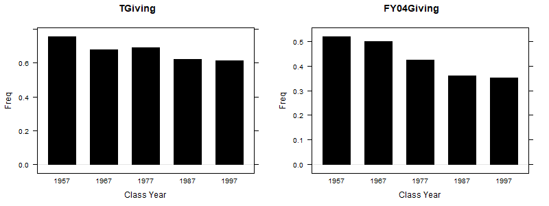
don$TGivingIND=cut(don$TGiving,breaks=c(-1,0.5,10000000),labels=FALSE)-1
mean(don$TGivingIND)
t5=table(don$TGivingIND,don$Class.Year)
t5
barplot(t5,beside=TRUE)
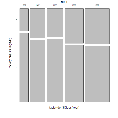
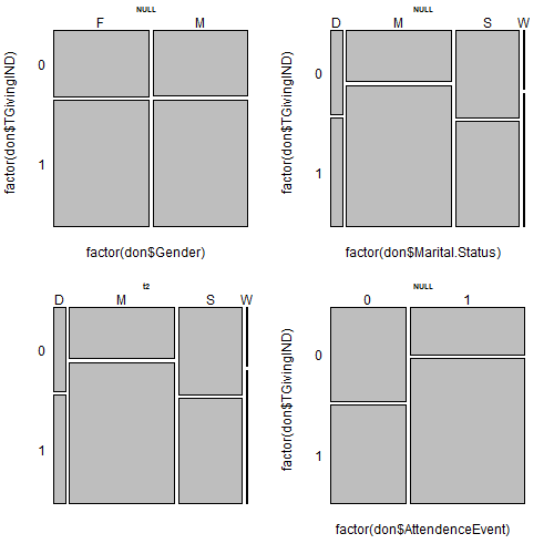
mosaicplot(factor(don$Class.Year)~factor(don$TGivingIND))
t50=tapply(don$TGivingIND,don$Class.Year,FUN=mean,na.rm=TRUE)
t50
p3=barchart(t50,horizontal=FALSE,xlab="Class Year",col="black", main="TGiving")
don$FY04GivingIND=cut(don$FY04Giving,c(-1,0.5,10000000),labels=FALSE)-1
t51=tapply(don$FY04GivingIND,don$Class.Year,FUN=mean,na.rm=TRUE)
t51
p4=barchart(t51,horizontal=FALSE,xlab="Class Year",col="black", main="FY04Giving")
grid.arrange(p3, p4, ncol = 2)
dev.copy(png,'alumni_annual_barplotfreq.png',width = 800, height = 300)
dev.off()
Nam Le
Risk and Asset Management Specialist for Buildings and Engineering Systems
My research interests include Operation Research and Applied Statistics for Asset Management of Buildings and Engineering Systems.